

Fascinating math works behind the scenes every time you open your digital audio files. Most users only ask, “Which is better, MP3 or FLAC?” However, a giant universe awaits you, stretching from the Nyquist Theorem to psychoacoustic models.
Our music listening habits have completely changed today. On this journey from vinyl records to CDs, and then to streaming platforms, digital audio has always been at the center. What’s more, it’s possible to get much more performance from your current hardware with the right settings.
Throughout this guide, I will blend science, test results, and my field experience. You will find every detail, from practical conversion commands with FFmpeg to Windows audio quality optimization. We will also lay the facts behind high-resolution audio (Hi-Res Audio) marketing on the table!
What Is Digital Audio? Basic Definition & Historical Context
Digital audio is created when you measure analog sound waves at specific intervals and convert them into numerical values. We call this process sampling. Audio files are not just a pile of data on their own. In fact, all multimedia content gains meaning by combining with images and text.
We record each measurement point as a number representing the amplitude of the sound at that moment. In the end, we are left with a massive sequence of numbers. This sequence is the form of sound that a computer can process.
This conversion process isn’t perfect. A phenomenon called quantization error creates tiny rounding mistakes while converting the analog signal to digital.
Fortunately, modern techniques reduce these errors to an almost inaudible level. The dithering technique, in particular, converts these errors into random noise. This way, your ear tolerates this noise much more easily.
| Concept | Explanation | Example Value |
|---|---|---|
| Sample Rate | The number of measurements taken per second | 44,100 Hz (CD quality) |
| Bit Depth | The precision level of each sample | 16-bit (65,536 levels) |
| Bitrate | The amount of data transferred per second | 1,411 kbps (CD stereo) |
| Number of Channels | The number of independent audio streams | 2 (Stereo), 6 (5.1 Surround) |
Sound Waves and Analog Representation: The Nature of a Continuous Signal
An analog audio signal is an electrical voltage that changes continuously over time. Your microphone picks up the pressure changes in the air and converts them into a signal with the same waveform.
The biggest advantage of this continuous signal is its infinite resolution. However, this is also its biggest disadvantage, because you add noise to the system with every copy you make.
In the analog world, the frequency spectrum is unlimited. But in practice, every circuit element acts like a cut-off filter. Therefore, harmonic distortion is inevitable in analog systems. Despite this, many audiophiles prefer the warmth of analog sound to digital.
When you do a waveform visualization, you can clearly see the smooth curves of the analog signal. The digital signal, on the other hand, resembles stair steps.
But don’t worry; with the correct resampling, these steps turn back into a completely smooth wave. Digital-to-analog converter (DAC) circuits perform exactly this transformation.
The Nyquist-Shannon Sampling Theorem: Why Is CD Quality 44.1 kHz 16-Bit?
The Nyquist-Shannon sampling theorem is the cornerstone of digital audio. So, the theorem states this: you want to capture a signal without errors.
Therefore, you must set your sampling rate to at least twice the highest frequency. The human ear can theoretically hear up to 20 kHz. Consequently, a rate above 40 kHz is sufficient.
So why exactly is the CD standard 44.1 kHz? This is an interesting story. In the 1970s, engineers recorded audio data onto video cassettes. In the PAL system, they took 3 samples per line. This corresponded to 44.1 kHz. Sony and Philips adopted this value as the Red Book standard.
Bit depth, on the other hand, determines how precisely each sample is measured. 16-bit means 65,536 different amplitude levels. This provides about 96 dB of dynamic range. It comfortably covers the difference between the quietest and loudest moments of a symphony orchestra.
The Digitization Process in Music: From Vinyl to the Streaming Era
The digitization process in music began with the commercial release of the CD in 1982. Until that day, analog records and cassettes were part of our lives.
With the CD, consumers experienced bit-perfect playback for the first time. Physical problems like the vibrations of a turntable needle or the wear of a tape head were no longer an issue.
At the end of the 1990s, MP3 compression fundamentally changed the music industry. You could now carry an album on a floppy disk. Of course, the price of this convenience was sacrificing some sound quality. However, thanks to the psychoacoustic model, the human ear does not notice most of the loss.
- 1982: They released the Compact Disc (CD), and 16-bit 44.1 kHz PCM became the standard.
- 1993: They published the MP3 format; thus, the era of lossy compression began.
- 2001: The Apple iPod and iTunes popularized the AAC codec.
- 2012: The IETF approved the Opus codec standard.
- 2020s: Spatial audio and Dolby Atmos music became widespread.
How Does Digital Audio Work? An In-Depth Analysis of PCM, Sample Rate & Bit Depth
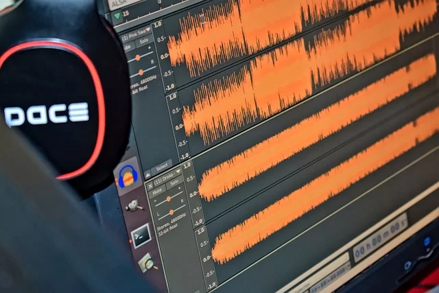
To grasp the working principle of digital audio technology, you must understand PCM modulation. I will explain the entire path from analog signal to digital data in detail. We will also examine critical subjects like quantization, quantization noise, and dithering.
The analog-to-digital converter (ADC) circuit takes the continuous signal coming from your microphone. It then takes measurements at specific time intervals.
The system stores each measurement result as a number in binary code. Later, the DAC converts this sequence of numbers back into a continuous signal. This cycle is the foundation of all systems.
In this process, sample rate and bit depth are vital. These two parameters directly determine the quality of your audio data stream.
A poorly configured system leads to inter-sample peak problems and distortion. Fortunately, you can eliminate these problems with the right configuration.
What Are PCM (Pulse Code Modulation) and LPCM?
Pulse code modulation is the most fundamental method for converting an analog signal to digital. In this method, you measure the amplitude of the signal at regular intervals.
You express each measurement as a number in the binary system. Almost all systems, from CDs to Blu-rays, use PCM, which stands for pulse code modulation.
LPCM, on the other hand, means linear PCM. In this format, we distribute the quantization levels linearly. This means each step represents an equal amplitude difference.
This makes reconstructing the signal extremely simple and error-free. The raw audio data you see inside a WAV file is actually in LPCM format.
PCM’s biggest advantage is its simplicity. Because we do not apply a compression algorithm, the processor load is minimal.
However, the disadvantage is the massive file sizes. One minute of stereo 16-bit 44.1 kHz PCM audio takes up about 10 MB. These byte sizes reveal just how bloated raw PCM data is. This is exactly why we need formats with a high digital audio compression ratio.
A Comprehensive Guide to Sample Rate and Bit Depth
The sample rate determines how many times you measure per second. Its unit is Hertz. 44,100 Hz means 44,100 measurements per second.
The higher this value, the higher the maximum frequency you can capture. However, going beyond the Nyquist limit is meaningless for the human ear.
Bit depth, on the other hand, determines the dynamic range. Each bit provides about 6 dB of additional dynamic range. Keep this formula in mind: Bit depth × 6 = approximate dynamic range (dB). 16-bit offers 96 dB, while 24-bit offers 144 dB of theoretical dynamic range.
| Sample Rate | Bit Depth | Maximum Frequency | Dynamic Range | Use Case |
|---|---|---|---|---|
| 8 kHz | 8-bit | 4 kHz | 48 dB | Telephone, VoIP codecs G.711 AMR |
| 22.05 kHz | 8-bit | 11 kHz | 48 dB | Old games, multimedia |
| 44.1 kHz | 16-bit | 22.05 kHz | 96 dB | CD, broadcast, podcast |
| 48 kHz | 24-bit | 24 kHz | 144 dB | Film, video, DVD |
| 96 kHz | 24-bit | 48 kHz | 144 dB | Studio recording, mixing |
| 192 kHz | 24-bit | 96 kHz | 144 dB | Archiving, mastering |
Quantization Error, Quantization Noise, and the Dithering Technique
When converting the signal to digital, you round each measurement to the nearest integer value. This rounding process creates quantization error.
The difference is added to the signal as quantization noise. At low bit depths, this noise reaches an annoying level. Think of 8-bit audio; you know that hiss.
The dithering technique solves this problem. Before rounding, you add very low-level random noise to the signal.
This way, the quantization error ceases to be periodic distortion. It transforms into a flat noise floor. Our ear tolerates constant noise much better than periodic distortion.
Dithering is indispensable in modern mastering. I personally prefer iZotope Ozone’s MBIT+ dither algorithm. However, FFmpeg’s default dither is also sufficient in most cases. This is exactly the answer to what dither is and how it affects sound quality.
32-Bit Float Audio: A Revolution in Studio Recording
The 32-bit float audio format is one of the most exciting developments of recent years. Unlike traditional integer formats, clipping is almost impossible in this format.
Even if the audio level exceeds 0 dBFS, the data is not lost. You can lower the level later during mixing and recover all the details.
The working principle of this format is quite clever. The system stores the number in two parts: the mantissa and the exponent, just like in scientific notation.
Thanks to this, you get an extraordinary dynamic range: 1528 dB! Of course, this is a theoretical value. In practice, your analog circuits use only a very small portion of this range.
I now use only 32-bit float in my recordings. Eliminating the need for audio level normalization is a huge advantage.
Explosion sounds, applause, or unexpected loud moments no longer ruin my recordings. Devices like the Sound Devices MixPre and Zoom F6 have brought this technology to the field.
The Difference Between Analog and Digital Audio: Comparative Advantages and Disadvantages
The difference between analog and digital audio has been the hottest topic of debate for years. Some defend the warmth of analog, while others champion the precision of digital. As someone who has worked in both worlds for years, I will present you with an objective comparison.
Analog systems process the signal continuously. For this reason, they theoretically offer infinite resolution. However, every circuit element adds noise, and every cable picks up interference.
Digital systems, on the other hand, store and transmit the signal error-free once it has been converted to digital. However, quantization error occurs during the conversion.
- Digital advantages: flawless copying, easy storage, fast access, noise immunity, and ease of editing.
- Analog advantages: natural frequency roll-off, unlimited theoretical resolution, and harmonic richness.
- Digital disadvantages: quantization error, Nyquist limit, and the risk of format obsolescence.
- Analog disadvantages: noise, generation loss, physical degradation, and limited dynamic range.
Signal Integrity and Noise Immunity
In terms of signal integrity, digital systems have an overwhelming superiority over analog systems. When you transmit digital data, you reconstruct the same signal on the receiver side.
Error correction mechanisms detect and correct transmission errors. In analog transmission, however, every cable and every connector adds a bit of noise to the signal.
When it comes to noise immunity, digital is also far ahead. Electromagnetic interference, ground loops, or power supply noise directly affects the analog signal.
Digital signals, however, are not affected by this interference up to a certain threshold. You either read the signal correctly or you do not read it at all.
| Criterion | Analog Audio | Digital Audio |
|---|---|---|
| Signal Integrity | Deteriorates with every copy | Copied infinitely without error |
| Noise Immunity | Low, open to interference | High, protected by error correction |
| Frequency Response | Natural roll-off, unlimited theoretical upper limit | Sharp cut-off at the Nyquist limit |
| Dynamic Range | 60–80 dB (consumer), 90 dB (professional) | 96 dB (16-bit), 144 dB (24-bit) |
| Storage | Physical medium, deteriorates over time | Digital file, infinite lifespan |
| Editing | Difficult, physical cutting and splicing | Extremely easy, non-destructive |
The Overwhelming Superiority of Digital in Copying and Archiving
Every time you copy an analog cassette, you experience generation loss. Each new generation is a little noisier and more distorted than the last.
But you can copy a FLAC file a million times if you wish. Every copy is identical to the original. This feature has revolutionized digital audio archiving and mastering.
In terms of archiving, digital formats also offer unparalleled advantages. Thanks to hard drives, cloud storage, and optical media, you can carry thousands of hours of recordings in the palm of your hand.
Furthermore, you can easily organize your archives thanks to information like metadata and ID3 tags. This is not possible in the analog world, however.
But digital archiving has its own unique risks. The obsolescence of file formats, the deterioration of storage media, and software incompatibilities are the main risks.
For this reason, you must store your important recordings in more than one format. Additionally, I recommend backing up this data in different physical locations. I personally back up my critical projects both on a local NAS and in the cloud.
Codec & Container Difference: The Anatomy of Audio Files
There are two fundamental concepts that confuse everyone stepping into the world of digital audio: codec and container.
Many people think MP4 is an audio format. However, MP4 is a container format. The audio inside it is encoded with AAC, MP3, or another audio codec component.
An audio codec is a software or hardware unit that compresses and decompresses raw PCM data. An encoder, on the other hand, compresses the audio itself.
The decoder, on the other hand, makes the compressed data playable again. The container holds the compressed audio data, metadata, and sometimes video together.
On the other hand, some formats appear as both a codec and a container. For example, a WAV file is both a container and a carrier of LPCM audio.
Similarly, OGG acts as a carrier for the Vorbis audio encoder. Moreover, this extension is a format in its own right.
What Is a Codec? The Audio Encoding and Decoding Process
An audio codec component is an algorithm that reduces raw PCM audio data to smaller sizes. The word codec comes from combining the words coder and decoder.
During encoding, the system analyzes the audio data. It discards unnecessary or inaudible information. It then efficiently packages the remaining data.
The codec choice determines the balance between sound quality and file size. Codecs using a lossless compression algorithm do not compromise sound quality. However, the compression ratio is low.
A lossy compression algorithm, on the other hand, produces much smaller files. But it permanently deletes some audio information. Which codec you choose depends entirely on your usage scenario.
Each codec has its own performance characteristic. Some codecs shine at low bitrate values, while others establish superiority at high bitrates.
For instance, the Opus codec offers quality equivalent to 128 kbps MP3 at 64 kbps. This difference stems from the algorithmic superiority in the codec design.
Audio File Container Formats: MKV, MP4, OGG, WebM
Container formats, also known as media muxers, hold audio and video streams together. A single container can hold multiple audio tracks, subtitles, and metadata at the same time. For example, an MKV file can simultaneously host both FLAC and AC-3 audio codecs.
Container choice becomes critical, especially when it comes to audio synchronized with video. Despite being the most common container, MP4 does not support every audio codec.
The OGG container is a favorite of the free software world. It is also ideal for the Vorbis and Opus codecs. MKV, on the other hand, is a universal container that accepts almost any codec.
| Container | Supported Audio Codecs | Metadata Support | Most Suitable Use |
|---|---|---|---|
| WAV | LPCM, uncompressed | Limited | Studio recording, archiving |
| MP4 | AAC, MP3, ALAC | Advanced | Video, podcast, mobile |
| MKV | FLAC, AC-3, DTS, PCM, Opus | Very advanced | Movie archive, Blu-ray |
| OGG | Vorbis, Opus, FLAC | Medium | Gaming, web, free software |
| WebM | Opus, Vorbis | Limited | Web streaming, HTML5 |
| FLAC (native) | FLAC | Advanced (Vorbis comment) | Music archive, audiophile |
Container Selection: Which Container Do You Use in Which Situation?
When choosing a container, ask these questions: What is your target platform? Which codecs will you use? Do you need metadata? You can select the ideal container based on the answers:
- For web audio streaming: Use the Opus codec in a WebM container. Moreover, almost all browsers support this combination.
- For a movie archive: Prefer the MKV container. It is the most flexible solution thanks to its support for multiple audio tracks, subtitles, and metadata.
- For mobile devices and social media: The MP4 container is ideal. What’s more, it provides excellent compatibility with the AAC codec.
- For studio and mastering: Use a raw WAV file. There is no compression or container complexity.
- For game engine integration: I recommend the OGG container. It offers low latency and quality compression.
The Complete Encyclopedia of All Digital Audio Formats and Codecs
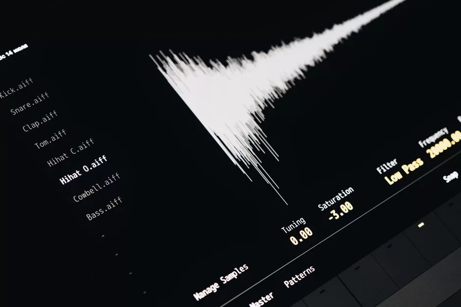
The world of digital audio formats is incredibly vast. Engineers designed each format to meet a specific need.
Now, we will examine all the important formats one by one, from WAV to MP3 and from FLAC to DTS.
When choosing a format, you evaluate three fundamental factors: sound quality, file size, and compatibility.
In a professional studio recording environment, quality is the priority. On mobile devices, storage and bandwidth are critical. This is why a different format stands out for each scenario.
- Uncompressed formats: WAV, AIFF, LPCM – highest quality, largest file size.
- Lossless compressed formats: FLAC, ALAC, WMA Lossless – up to 50% size savings without sacrificing quality.
- Lossy compressed formats: MP3, AAC, Ogg Vorbis, Opus – high compression ratio, controlled quality loss.
- Surround formats: AC-3, DTS, Dolby TrueHD – for multi-channel cinema and home theater.
- Speech codecs: G.711, AMR, Opus speech mode – low bandwidth, low latency.
Uncompressed Format: WAV (Waveform Audio File Format) and LPCM
Microsoft and IBM developed the WAV file format in 1991. It contains raw LPCM audio data inside. Because they apply no compression, the sound quality is completely original.
However, the price of this quality is massive file sizes. One hour of stereo 16-bit 44.1 kHz WAV recording takes up about 635 MB.
The biggest advantage of the WAV format is its universal compatibility. Whether you use Windows, Mac, or Linux, every system can play WAV files.
Furthermore, all digital audio workstation software supports the WAV format natively.
However, WAV has its disadvantages too. The 4 GB file size limit can pose a problem for long recordings. Also, metadata support is quite limited. You will experience compatibility issues when you want to add an ID3 tag.
The answer to whether WAV or MP3 is better depends on your intended use. For professional work, WAV is suitable. For daily listening, on the other hand, prefer MP3 or AAC.
Lossless Compressed Formats: FLAC, ALAC, and WMA Lossless
FLAC (Free Lossless Audio Codec), as the name suggests, is completely free and open source.
It reduces the size of PCM audio data by about 40–60 percent. However, it does not lose a single bit. As a result of decompression, you get audio bit-for-bit identical to the original WAV.
ALAC (Apple Lossless Audio Codec), on the other hand, is the lossless format of the Apple ecosystem. It offers performance similar to FLAC.
However, thanks to its seamless integration with Apple devices, it is ideal for iPhone and Mac users. The WMA Lossless format is Microsoft’s solution in this area.
| Format | Compression Ratio | Open Source | Platform Support | Best Use |
|---|---|---|---|---|
| FLAC | 40–60% reduction | Yes | All platforms | Music archive, audiophile listening |
| ALAC | 40–60% reduction | Yes (since 2011) | Apple, limited others | Apple ecosystem |
| WMA Lossless | 40–60% reduction | No | Windows, limited others | Old Windows systems |
Lossy Compressed Formats: MP3, AAC, Ogg Vorbis, Opus
MP3 is the first format that comes to mind when talking about lossy audio compression. The Fraunhofer Institute developed MP3 compression technology in the 1990s.
What’s more, this technology completely discards inaudible frequencies using psychoacoustic models. Even at a 128 kbps bitrate, it offers satisfactory quality for most listeners.
Engineers designed AAC (Advanced Audio Codec) as the successor to MP3. It uses more efficient psychoacoustic encoding. At the same bitrate, it offers noticeably better sound quality than MP3. Moreover, platforms like YouTube, Apple Music, and Nintendo Switch prefer AAC.
Ogg Vorbis is a completely open-source and patent-free lossy codec. Game developers and free software projects that want to avoid MP3’s patent issues prefer it.
The Opus codec, on the other hand, is the most advanced lossy codec of the modern era. It shows excellent performance at all bitrates from 6 kbps to 510 kbps.
| Codec | Year of Release | 128 kbps Quality | Low Bitrate Performance | Patent Status |
|---|---|---|---|---|
| MP3 | 1993 | Good | Weak (below 64 kbps) | Patented (expired) |
| AAC | 1997 | Very good | Moderate (below 48 kbps) | Patented |
| Ogg Vorbis | 2002 | Very good | Good (below 48 kbps) | Patent-free |
| Opus | 2012 | Excellent | Excellent (even at 6 kbps) | Patent-free |
High-Resolution Format: DSD (Direct Stream Digital)
DSD, Direct Stream Digital, uses a completely different approach from PCM. It records the audio signal as a single-bit, very high-speed stream instead of multi-bit samples. A typical DSD signal flows at 2.8224 MHz, which is 64 times CD quality.
DSD’s theoretical advantage is its simplicity. Quantization error and filtering requirements in PCM are minimized in DSD.
However, in practice, the audibility of this advantage is quite controversial. Additionally, DSD files are extremely difficult to edit. Most digital audio workstation software cannot process DSD directly.
I personally think DSD is valuable as an archive format. However, it is not practical for daily use. The file sizes are astronomical, and portable device support is limited.
First, you should learn the PCM audio format. As a result, you will understand the different approach offered by DSD technology much better.
Surround and Cinema Formats: AC-3 (Dolby Digital), E-AC-3, DTS, Dolby TrueHD
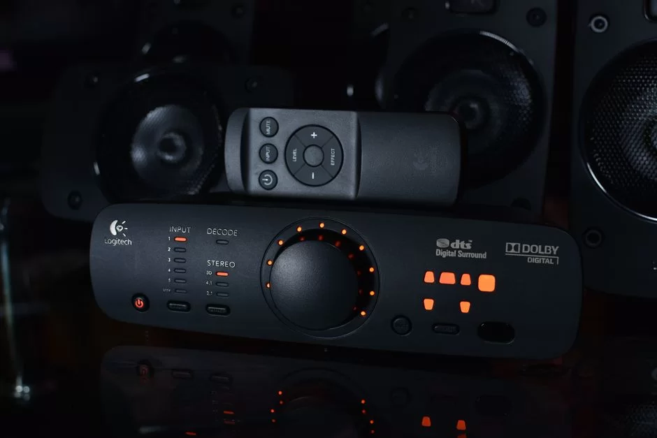
If you ask what AC-3 and DTS are, I would say they are the heart of the cinema experience. Engineers designed these formats specifically for multi-channel surround systems.
AC-3, or Dolby Digital, compresses audio with lossy compression up to 5.1 channels. It is also the standard on DVDs and many broadcasting platforms.
Dolby TrueHD and DTS-HD Master Audio, on the other hand, are lossless surround formats. Found on Blu-ray discs, these formats bring studio-quality multi-channel audio to your home.
Developers built the spatial audio API (Microsoft Spatial Sound) on this foundation. Moreover, they added technologies like Dolby Atmos on top of it.
| Format | Compression | Maximum Channels | Bitrate | Platform |
|---|---|---|---|---|
| AC-3 (Dolby Digital) | Lossy | 5.1 | 384–640 kbps | DVD, broadcasting |
| E-AC-3 (Dolby Digital Plus) | Lossy | 7.1 | Up to 1.7 Mbps | Streaming, Blu-ray |
| DTS | Lossy | 5.1 | 768–1536 kbps | DVD, Blu-ray |
| Dolby TrueHD | Lossless | 7.1 | Up to 18 Mbps | Blu-ray |
| DTS-HD Master Audio | Lossless | 7.1 | Up to 24.5 Mbps | Blu-ray |
Speech and VoIP Codecs: G.711, G.722, AMR, Opus (Speech Mode)
Codecs designed for speech communication have different priorities from music codecs. What is critical here is low latency and low bandwidth. VoIP codecs like G.711 and AMR target the frequency range of human speech.
G.711 is the fundamental codec of telephone networks. It uses a constant bitrate (CBR) of 64 kbps and creates an extremely low processor load.
G.722, on the other hand, offers wideband audio and can transmit frequencies up to 7 kHz. Engineers have optimized the AMR codec family for mobile networks. It operates with a variable bitrate (VBR).
The speech mode of the Opus codec leaves all these traditional codecs behind. It simultaneously supports both narrowband and fullband speech.
Moreover, it can dynamically switch to music mode. This is why modern communication applications like Discord, WhatsApp, and Telegram prefer Opus.
Format Selection Table: Which Format Should You Use in Which Situation?
| Usage Scenario | Recommended Format | Alternative Format | Reason |
|---|---|---|---|
| Studio recording and mixing | WAV (24-bit 48 kHz) | 32-bit float WAV | Highest quality, ease of editing |
| Music archive (audiophile) | FLAC | ALAC (Apple users) | Lossless, 50% space savings |
| Mobile music listening | AAC (256 kbps VBR) | Opus (192 kbps) | High quality, low size |
| Podcast broadcasting | AAC (128 kbps) | MP3 (192 kbps) | Wide compatibility, sufficient quality |
| Web streaming | Opus (96–128 kbps) | AAC | Best low bitrate performance |
| Game audio engine | OGG Vorbis | Opus | Patent-free, low CPU load |
| Film and surround | AC-3 / E-AC-3 | DTS | Multi-channel support, wide compatibility |
| VoIP and conferencing | Opus (speech mode) | G.722 | Low latency, high quality |
The Science of Audio Compression Algorithms: An In-Depth Analysis of Lossy and Lossless Methods
Audio compression algorithm design is one of the most elegant fields of computer science. In this field, entropy coding, predictive coding, and psychoacoustic models work together.
Every compression algorithm aims to detect and eliminate redundancies in the data. It also cleans out components that the human ear cannot hear.
Lossless compression reduces file size by finding statistical repetitions in the data. Lossy compression is much more aggressive; it discards inaudible frequencies.
Understanding the difference between the two directly affects your format choice, because in lossy compression, you can never recover the data you discarded.
Lossless Compression Algorithms: Huffman, RLE, and Predictive Coding
Huffman coding is the entropy coding method we use most frequently. It assigns short codes to frequently repeated values and long codes to rare values. Thus, the total number of bits decreases. Formats like FLAC and ALAC use Huffman-like variable-length coding.
RLE, run-length encoding, is one of the simplest lossless compression algorithms. If the same value repeats consecutively, it stores that value and the repetition count.
It is especially effective in sections of silence. Predictive coding goes one step further. It predicts the value of the next sample and stores only the prediction error.
The LZW algorithm, on the other hand, is a dictionary-based method we use in formats like GIF and TIFF. Although it is not very common in audio, it appears as a sub-component in some lossless codecs. The common point of all these methods is this: when you compress and decompress audio, you get an exact, bit-for-bit copy of the original data.
Psychoacoustic Model and Auditory Masking: The Working Principle of MP3 and AAC

A psychoacoustic model is a mathematical simulation of the human hearing system. This model calculates which frequencies you cannot hear under which conditions.
For example, a loud bass sound hides lower-intensity sounds at nearby frequencies with a masking effect. The codec does not record these masked sounds. This way, it saves bandwidth.
Auditory masking is of two types: frequency masking and temporal masking. In frequency masking, a strong signal at a close frequency makes a weak signal inaudible.
In temporal masking, on the other hand, you do not perceive low-intensity sounds that come just before or after a louder sound.
The MP3 format eliminates some frequencies. Masking principles specifically explain why this happens.
MP3 compression divides the audio into 32 sub-bands and performs a separate masking analysis for each band. Thanks to sub-band coding, it processes each frequency region independently.
It then packages the remaining data with entropy coding. AAC, on the other hand, uses more sub-bands and a more advanced psychoacoustic model.
CBR, VBR, and ABR Encoding Modes: Which One Do You Use When?
Constant bitrate (CBR) uses the same amount of data for every second. This method is simple, and you can predict the file size precisely.
However, quality drops in complex passages. In simple passages, you waste bits. It is ideal for situations requiring a constant bandwidth, such as data streaming and live broadcasting.
Variable bitrate (VBR), on the other hand, dynamically adjusts the bitrate according to the complexity of the audio. It uses a low bitrate in quiet sections and increases it in intense passages. This way, it offers much better quality at the same average size. Consequently, you should always prefer VBR for a music archive.
Average bitrate (ABR) is a compromise between CBR and VBR. It targets a specific average bitrate. However, it allows fluctuation when necessary. It is suitable for those who want to estimate the file size. It also appeals to those who do not want to sacrifice quality.
| Mode | File Size | Quality Consistency | Best Use |
|---|---|---|---|
| CBR (Constant) | Fully predictable | Variable, lower in complex parts | Live broadcast, VoIP |
| VBR (Variable) | Unpredictable | High and consistent | Music archive, local storage |
| ABR (Average) | Roughly predictable | Good, higher than CBR | Streaming services, podcast |
Conversion Between Formats, Metadata & ID3 Tag Management (A Practical Guide with FFmpeg)
FFmpeg is the Swiss Army knife of the digital audio world. With this tool, you can perform tasks like audio conversion, metadata editing, and even live streaming. Do not let its command-line operation scare you. Once you learn it, it gives you incredible control over your DSP settings.
The most common mistake you make when doing audio conversion is converting with default values without understanding the codec parameters. FFmpeg gives you the ability to control every parameter. The bitrate, sample rate, number of channels, and codec selection are entirely in your hands.
Also, metadata management is at least as important as sound quality. A music archive you have not tagged correctly turns into inextricable chaos over time. Thanks to the ID3 tag, you embed information like artist, album, year, and genre into your files.
Audio Conversion with FFmpeg: Basic Commands and Parameters
To convert from WAV to FLAC with FFmpeg, use the following command:
ffmpeg -i input.wav -c:a flac -compression_level 8 output.flacThis command takes the input file and produces output with the FLAC codec at maximum compression level. The parameter to note is -c:a, which stands for codec audio. If you specify the wrong codec, FFmpeg gives you an error.
When you want to convert to MP3, it is better to determine the quality with VBR:
ffmpeg -i input.wav -c:a libmp3lame -q:a 2 output.mp3Here, the -q:a 2 parameter means high-quality VBR encoding. A value of 0 is the highest quality, and 9 is the lowest. I generally use 2 for music and 5 for podcasts.
You perform conversion with the Opus codec like this:
ffmpeg -i input.wav -c:a libopus -b:a 128k output.opusOpus’s biggest advantage is that it offers excellent quality even at low bitrates. At 64 kbps, it is more than enough for speech. In short, it delivers surprisingly good results for music as well.
ID3 Tags and Metadata Management: Bulk Tag Editing with FFmpeg
Audio tag management is essential for a well-organized music archive. Use the following command to add metadata with FFmpeg:
ffmpeg -i input.flac -c copy -metadata title="Track Name" -metadata artist="Artist" -metadata album="Album" output.flacThe -c copy parameter allows you to add only metadata without re-encoding the audio. This way, there is no quality loss, and the process completes in seconds.
Also, you can write a small script for bulk tag editing. Alternatively, you can call FFmpeg inside a loop.
The ID3 tag is particularly common for MP3 files. It has two main versions: ID3v1 and ID3v2. ID3v1 uses a fixed 128-byte field at the end of the file.
ID3v2, on the other hand, is located at the beginning of the file. It also offers much richer metadata support, such as album art and lyricist information.
Digital Audio Level Normalization and Dynamic Range Preservation
Digital audio level normalization is the process of equalizing the perceived loudness of different recordings. Preserving the dynamic range is critical when doing this. Simply boosting the entire audio leaves the dynamic range as it is. However, it equalizes the sound level.
A more advanced method is LUFS (Loudness Units relative to Full Scale) based normalization. This method accounts for how the human ear perceives sound. Therefore, the EBU R128 and ITU BS.1770 standards are the authorities on this subject.
To perform LUFS normalization with FFmpeg, use the loudnorm filter:
ffmpeg -i input.wav -c:a libmp3lame -b:a 320k -filter:a loudnorm=I=-14:TP=-1 output.mp3This command sets the integrated loudness value to -14 LUFS. It sets the true peak value to -1 dBTP. Among the best audio settings for podcasts, you often see these values.
Improving Digital Audio Quality: Software and Hardware Optimization
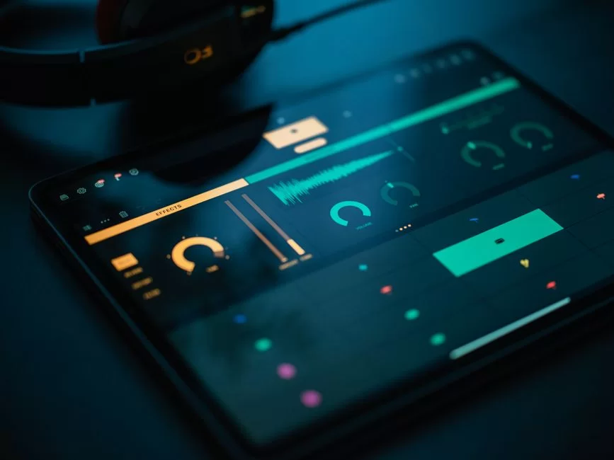
How to improve digital audio quality is perhaps the question I encounter most frequently. The answer is more complex than you might think.
Many factors affect quality along the entire audio chain architecture. Every component, from the operating system’s audio engine settings to the cable you use, is important.
Windows users need to be especially careful. The default Windows Audio Engine merges all audio streams in a mixer and resamples them. This process can degrade sound quality.
Fortunately, you can bypass this problem by using WASAPI Exclusive Mode or an ASIO driver.
On the hardware side, you should use an external DAC chip, because this investment offers much cleaner sound than an onboard sound card.
You should make your selection by looking at the SINAD measurement and Total Harmonic Distortion (THD+N) values. When making a USB DAC vs. PCI-e sound card comparison, remember this: USB DACs generally offer cleaner power isolation.
- USB DAC: external power supply, portability, electrical isolation advantage.
- PCI-e Sound Card: lower latency, internal installation, more stable driver support.
- Onboard sound card: cost-free, but limited SINAD and open to electromagnetic interference.
Does the Windows Audio Mixer Degrade Sound? A Bit-Perfect Solution with WASAPI and ASIO
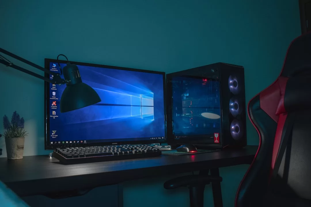
Unfortunately, the answer to whether the Windows audio mixer degrades sound is yes. The default Windows Audio Session API collects all audio streams. It then converts them to a common sample rate.
A quality loss occurs during this resampling. Moreover, system sounds can mix into your music.
Let me explain, step by step, how to use WASAPI Exclusive mode:
- Download a WASAPI-compatible player like Foobar2000.
- For the Foobar2000 WASAPI setup, install the output component from the official plugin page.
- In the player settings, select “WASAPI (event): Your DAC” as the output device.
- In this mode, you only play the music. You block all other system sounds.
- The player automatically uses the sample rate your DAC supports.
The ASIO driver, on the other hand, offers even lower latency. It is the standard for professional studio applications. To install it, first install the ASIO driver from the manufacturer of your audio interface. However, for built-in sound cards, the ASIO4ALL driver is a temporary solution.
Fixing Audio Stuttering Caused by DPC Latency
DPC latency (Deferred Procedure Call) is the most insidious cause of audio stuttering. If a driver occupies the CPU for too long, you cannot fill the audio buffer in time. Consequently, crackles and stutters occur. This problem is especially annoying in games and live audio processing applications.
With the LatencyMon latency checker tool, you can easily detect which driver is causing the problem. Run the program and wait until you experience an audio stutter.
In the report, you will see the driver with the highest DPC time. Usually, the culprit is a network driver, a graphics card, or a power management driver.
Increasing the audio buffer size is also a temporary solution. If you ask what buffer size is, it is the number of samples the sound card collects beforehand to process. A larger buffer means fewer stutters.
However, it introduces more latency. For gaming, 128–256 samples are ideal; for music production, 64–128 samples.
Audio Latency and Quality Settings for Gamers and Podcasters
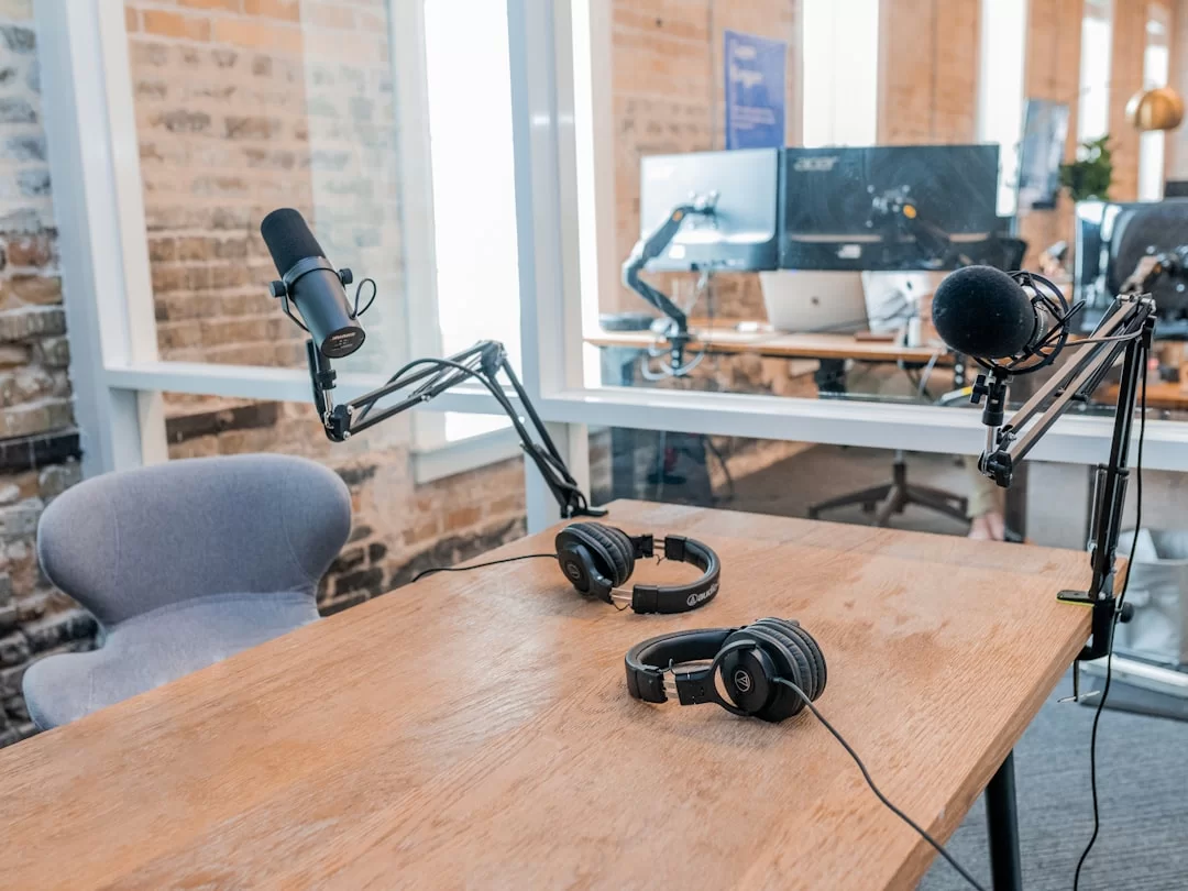
You must optimize competitive FPS game audio settings to hear your opponents’ footsteps. The most critical factor here is the choice of virtual surround software. An HRTF algorithm for virtual surround allows you to position the direction of sounds correctly.
I recommend the following settings for reducing audio latency in games:
- Turn off all effects, EQs, and surround simulations in the sound card control panel.
- Set the sample rate to 48 kHz and the bit depth to 24-bit. Keep the buffer size at 128 samples or lower.
- Disable all options under the “Enhancements” tab in the Windows sound mixer.
- Select “Stereo” or “Headphone” mode in the in-game audio settings; leave virtual surround to the game’s own engine.
- If you compare Windows Sonic with Dolby Atmos, Sonic offers lower latency in competitive games.
The best audio settings for a podcast are completely different. Here, latency is not important. However, sound quality and noise reduction are critical.
You should learn to use Nvidia Broadcast noise removal settings. In other words, this tool, or RTX Voice, will dramatically improve your broadcast quality.
You can use AI-powered audio cleaning programs. This way, you can easily remove keyboard sounds, fan noise, and room echo.
If you are using wireless headphones, pay attention to some details. To reduce latency, choose devices that support LDAC or aptX HD.
Windows’ inefficient AAC encoding causes poor Bluetooth AAC performance. Third-party drivers are available for LDAC usage on Windows.
However, you may experience stability issues. For a wireless headphone lip-sync problem, manually correct the audio delay setting in your player.
Spotify, Apple Music, Tidal, and YouTube Audio Quality Settings
Every streaming platform has its own audio quality settings. For the best Spotify audio quality, select “Very High.” This option corresponds to Ogg Vorbis 320 kbps. Apple Music, on the other hand, offers lossless and high-resolution audio in the ALAC format.
If you ask how to improve YouTube audio quality, the answer is limited. YouTube compresses audio in Opus or AAC format.
Increasing the video resolution also increases the audio bitrate. If you want to test Tidal’s bit-perfect playback, FLAC options are available in the platform’s HiFi Plus tier.
| Platform | Highest Quality | Codec | Bitrate / Format | Lossless Support |
|---|---|---|---|---|
| Spotify Premium | Very High | Ogg Vorbis | 320 kbps | No |
| Apple Music | Hi-Res Lossless | ALAC | 24-bit 192 kHz | Yes |
| Tidal HiFi Plus | MQA / FLAC | FLAC, MQA | 24-bit 192 kHz | Yes |
| YouTube Premium | High | Opus / AAC | 256 kbps (estimated) | No |
| Amazon Music HD | Ultra HD | FLAC | 24-bit 192 kHz | Yes |
High-Resolution Audio (Hi-Res): Science, Myths, and Practical Value
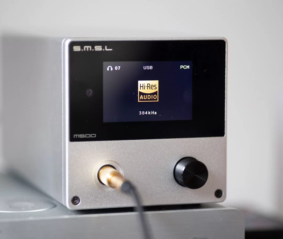
High-Resolution Audio (Hi-Res Audio) marketing has turned into a huge craze. This trend forces consumers to download unnecessarily large files.
Marketers present the 24-bit 192 kHz label as if it is a quality guarantee. However, the truth is very different. Now, let us look at the real value of Hi-Res audio in light of research.
We can give a simple answer to what Hi-Res audio is. Namely, we consider any recording that exceeds CD quality—meaning 16-bit 44.1 kHz—as Hi-Res.
This generally means 24-bit 96 kHz or higher. However, whether these extra bits and samples create an audible difference is a completely separate matter.
Is 24-Bit 192 kHz Really Audible? What Do Scientific Studies Say?
Organizations like the AES and ITU have repeatedly researched whether 24-bit 192 kHz is audible. The result is clear: experts conduct controlled blind tests (ABX tests). However, very few participants can distinguish between the two sound qualities under these conditions. In other words, you cannot hear the difference.
Human ear hearing limits are a determining factor for sound quality. A healthy young ear can theoretically hear the 20 Hz–20 kHz range.
This range narrows as age advances. A 44.1 kHz sampling rate captures frequencies up to 22.05 kHz without error. Why 192 kHz? The answer is simple: marketing.
In terms of bit depth, 16-bit offers a 96 dB dynamic range. The difference between the background noise of a concert hall and its loudest moment is about 80 dB.
So, 16-bit comfortably covers this difference. The extra dynamic range provided by 24-bit is useful only in a studio recording environment, during mixing.
The Hi-Res Audio Playback Chain: Bit-Perfect DAC, Headphones, and Recording
If you still want to listen to Hi-Res audio, every link in your playback chain must support this resolution. Your DAC must support at least 24-bit 192 kHz. The frequency range of your headphones must extend above 20 kHz.
Bit-perfect playback gains importance at this point. A bit-perfect signal path means the audio data undergoes no alteration until it reaches the DAC.
On Windows, you can achieve this only with WASAPI Exclusive Mode or ASIO. On macOS, on the other hand, CoreAudio automatically provides bit-perfect playback.
Jitter and clocking errors can also cause problems in a Hi-Res chain. A quality DAC chip minimizes these problems with a precise clock circuit.
But remember: even if you set up a perfect chain, the sound you hear will be no different from CD quality, because the limit is not in the equipment but in your ears.
Authorities to Guide You on Your Digital Audio Journey
You may want to gain in-depth knowledge about digital audio technologies. In that case, examine the following up-to-date and authoritative sources, because these platforms set the industry standards.
- Opus Codec Official Documentation – You can find all the technical details and interactive demo examples of the modern, patent-free audio codec compliant with IETF standards here.
- Hydrogenaudio Community Wiki – It offers the most up-to-date and in-depth, user-focused technical information on audio compression, codec comparisons, and blind test (ABX) results.
- FFmpeg Official Complete Documentation – The most detailed explanations of all the audio conversion and processing commands we used in the article are located here.
- DAFX: Digital Audio Effects – It is the official address of a globally accepted reference book and research conference on audio processing, digital signal processing, and effects.
- Sound On Sound Technical Articles – It is one of the most respected publications on professional audio engineering, recording techniques, and software reviews.
10 Critical Questions About the World of Digital Audio
What is digital audio and what are its formats?
What is the difference between lossy and lossless audio compression?
What is the difference between a codec and a container?
Which is better, WAV or MP3?
What is FLAC, and what is its difference from MP3?
What is the AAC format, and what is its difference from MP3?
What is the Opus codec, and why is it important?
Why is CD quality 44.1 kHz 16-bit?
What is the best digital audio format?
Does Hi-Res Audio (24-bit 192 kHz) really make a difference?
Conclusion: The Final Decision Guide for Your Digital Audio Journey
Throughout this guide, we covered everything from the fundamentals of digital audio to the most complex codec algorithms. You now know that there is no single answer to which is the best digital audio format. Every format serves a specific purpose. Use FLAC for archiving, AAC for mobile listening, Opus for the web, and WAV for the studio.
The most critical step regarding Windows sound quality improvement settings is this: enable bit-perfect playback with WASAPI Exclusive Mode or ASIO. You must accept that the audio mixer degrades sound and set up a professional signal path. Once you learn how to configure sound card settings, you will get much more performance from your current hardware.
Remember: perfect sound is the sound that satisfies your ears, not measurement devices. Apply what you learned in this guide to your own system. Do ABX tests, and most importantly, enjoy the music. Audio engineering is not a destination; it is a journey of continuous learning.

Be the first to share your comment